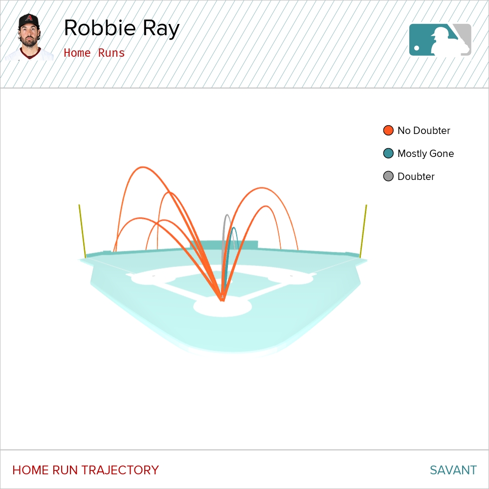
The latest feature added to Baseball Savant focuses on one of baseball’s most exciting plays: the home run. However, its creator, Daren Willman, tweeted, “Not all home runs are created equal.”
Not all home runs are created equal… Check out our new @statcast leaderboard for home runs. Click each player row and it lets you see which home runs would go out if it was hit at another stadium. https://t.co/u3mWUxlAVKpic.twitter.com/HRHFnQAMeA
The leaderboard’s startup screen shows all those batters in 2020 who hit at least one long ball that would have been a home run in at least one of Major League Baseball’s 30 ballparks.
On August 9, before any of the day’s games have been played, Yankees slugger Aaron Judge is Major League Baseball’s home run leader with eight. In the Home Runs Leaderboard, if you click anywhere on a player’s row except on his name, details on all his homers in the season you choose will appear, each homer listed on a separate row.
Click on Judge’s row. Below his name should beS a table showing those ballparks where each long ball that Judge hit on the given date will be a homer. For example, on August 8 in Tampa Bay, the first long ball that Judge hit (against Sean Gilmartin) would have been a four-bagger in every ballpark, but the second long ball he hit (against Nick Anderson) would have been a homer in only 18 parks — video.
Therefore, for a long ball to qualify for (be included in) the Home Runs Leaderboard it must have been able to be a home run in at least one MLB stadium even if it was not a homer in the ballpark in which it was hit. Those batted balls are labelled as “Doubters,” “Mostly Gone,” or “No Doubters.”
If a batted ball would be a homer in fewer than 8 ballparks, it is a “doubter.”
If it would be a homer in 8 to 29 parks, it is “mostly gone.”
If would be a home run in every stadium, it is a “no doubter.”
That is why if you sum those three columns (“Doubters,” “Mostly Gone,” “No Doubters”) the total could be less than what is in the “Actual HR” column, which is the total number of homers the player hit, as occurs with Fernando Tatis Jr.’s numbers. He had six actual homers, but one “doubter,” three “mostly gone,” and six “no doubters.”
Finally, home run data is available for batters, pitchers, and teams for both 2019 and 2020.
Here is a sample of the kinds of questions that Savant’s Home Runs Leaderboard can answer.
Which player’s has the most “could-be” homers that could only be a home run in one stadium?
This is fascinating. Only 3 batted balls from Kris Bryant could have been a home run. And each of those would only be a HR in exactly 1 park.
Which Mets’ player has hit the most actual and “almost” homers so far in 2020? Notice that one of Davis’ “homers” was a non-homer. I label that one a “Could Be” homer.
In 2020, which pitcher have given up the most “no doubters?”
The Home Runs Leaderboard is a great resource with eye-catching visuals for statistically-minded baseball fans. One thing that could make it even better is if you could get team data by both division and league. For example, now if I select “Mets” and “Pitchers,” I only get the results for the qualifying Mets pitchers.
In my first post on high-ball pitchers, I presented the top 10 high-ballers in 2019. On the bottom of the list based on the number of high-balls thrown was Astros starter Jordan Lyles, but his high-ball pitch percent of 28.4% pushed him into the two-spot. Given that the League average in 2019 was 16.8%, Lyles was more than 50% above average.
The strike zone has changed over the years. According to the OFFICIAL BASEBALL RULES, 2019 Edition,
The STRIKE ZONE is that area over home plate the upper limit of which is a horizontal line at the midpoint between the top of the shoul- ders and the top of the uniform pants, and the lower level is a line at the hollow beneath the kneecap. The Strike Zone shall be determined from the batter’s stance as the batter is prepared to swing at a pitched ball.
To appreciate what a high pitch is you need to know the strike zone’s dimensions.
Mike Fast wrote that there are two ways to dimension the strike zone.
One is to use fixed heights for the top and bottom boundaries of the zone for all batters, regardless of the height or stance of the batter. The most commonly used fixed heights are 1.5 feet for the bottom of the zone and 3.5 feet for the top of the zone.
As the second way involves the statistical technique of normalization, it will not be covered in this post. Those mathematically inclined can find an explanation here.
As Fast’s article was published in 2011, I checked the strike zone a second way. Statcast’s “Plate Z” setting shows a pitch’s height. In 2019, the average height of a pitch in the high-ball zone was 3.65 feet. In all zones, the average height was 2.25 feet. Since 2015, the average heights have been 2.25, 2.26, 2.41, 2.25, and 2.25, so they have been almost identical in four of the past five years.
Lindor’s homer, his 18th, was hit off a pitch 3.53 feet high and was the only homer he hit that season off a pitch at least three above the plate. In 2018, the average pitch height of his homers was 2.16 feet.
Every year since 1956 at least one pitcher has won the Cy Young Award starting with the Brooklyn Dodgers’ Don Newcombe. Many questions can be asked. How many pitchers won the award more than once? Which pitchers achieved that feat? Who won it the most times?
In this post, I focus on just one question: How many players won the Cy Young Award? I will share how I got the answer using the R programming language. I will also be using both RStudio and Sean Lahman’s Baseball Database, an excellent resource. A basic familiarity with both R, dplyr, and RStudio is assumed. (Note: As you progress through this post, have RStudio open.)
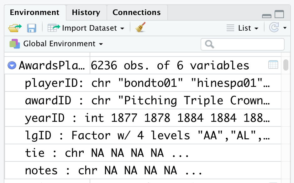
The database contains multiple files in table format. The table containing the player awards data is AwardsPlayers.RData. It has six variables:
playerID       Player ID code
awardID        Name of award won
yearID         Year
lgID           League
tie            Award was a tie (Y or N)
notes          Notes about the award
What AwardsPlayers.RData does not have are the players’ names though it has each Player’s ID. Their names are in People.RData. The People table contains 24 variables. In the partial display of its variables, notice that it too contains playerID.
playerID       A unique code asssigned to each player.
birthYear      Year player was born
birthMonth     Month player was born
birthDay       Day player was born
birthCountry   Country where player was born
birthState     State where player was born
birthCity      City where player was born
nameFirst      Player's first name
nameLast       Player's last name
weight         Player's weight in pounds
height         Player's height in inches
bats           Player's batting hand (left, right, or both)
throws         Player's throwing hand (left or right)
Fortunately, the playerID field links together the data in the tables.
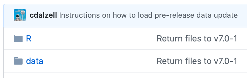
For this tutorial, you need to download from Lahman’s database the “2019 – R Package“. When the webpage appears, click “data.”
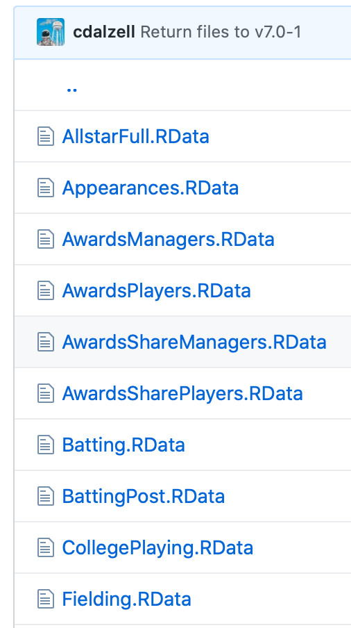
You will see a list of downloadable files. The files are in RData format, a format created for use in R. For this tutorial, download these two files: AwardsPlayers.RData and People.RData. The latter is not shown in the image below, which contains a partial file list.
After you click AwardsPlayers.RData, what is shown below will appear. Click View Raw. The file will download to your device. (Note: The way I show you to do something in this tutorial is often not the only way to do it.)
Click the downloaded file, which in this case is AwardsPlayers.RData. On my Mac, it downloaded into the Downloads folder.
When this appears, click Yes.
This should appear in your RStudio Console:
load(“/Users/Home/Downloads/AwardsPlayers.RData”
Here is how the AwardsPlayers.RData looks in RStudio’s Global Environment. It is now available for you to work on.
Now, in RStudio the two downloaded tables are R data frames. Next, I created an R Markdown file and made copies of both data frames.
AP <- AwardsPlayers
P <- People
Merge AP and P into a new data frame: AP_P. The column common to both, playerID, serves as the link.
AP_P <- merge(AP, P, by="playerID")
View the merged data frame’s variables.
glimpse(AP_P)
To view the data, while in the Console type
View(AP_P).
Activate the Tidyverse library, reduce the number of columns, and display the last 10 rows. Note: If you have not used it before, you may need to install it using the R code on the next line.
Select five columns in AP_P, and display the last 10 rows in AP_P.
nameFirst<chr>
nameLast<chr>
playerID<chr>
yearID<int>
awardID<chr>
6227
Ryan
Zimmerman
zimmery01
2010
Silver Slugger
6228
Ryan
Zimmerman
zimmery01
2011
Lou Gehrig Memorial Award
6229
Ryan
Zimmerman
zimmery01
2009
Silver Slugger
6230
Richie
Zisk
ziskri01
1981
TSN All-Star
6231
Richie
Zisk
ziskri01
1974
TSN All-Star
6232
Barry
Zito
zitoba01
2012
Hutch Award
6233
Barry
Zito
zitoba01
2002
Cy Young Award
6234
Barry
Zito
zitoba01
2002
TSN Pitcher of the Year
6235
Barry
Zito
zitoba01
2002
TSN All-Star
6236
Ben
Zobrist
zobribe01
2016
World Series MVP
The next step is to combine the nameFirst and nameLast columns in a new column, fullname. The paste function automatically inserts a space between the names.
In this table only the last eight observations are shown.
Go into the View window and set the settings you see below in the first row. Notice that the last year for the Cy Young Award is 2017, thus two years are missing.
Partial screenshot of View window
Add the missing data to the AP dataset.
AP <- add_row(AP, playerID = "degroja01", awardID = "Cy Young Award", yearID = 2018, lgID = "NL", tie = "NA", notes = "P")
AP <- add_row(AP, playerID = "snellwa01", awardID = "Cy Young Award", yearID = 2018, lgID = "AL", tie = "NA", notes = "P")
AP <- add_row(AP, playerID = "degroja01", awardID = "Cy Young Award", yearID = 2019, lgID = "NL", tie = "NA", notes = "P")
AP <- add_row(AP, playerID = "verlaju01", awardID = "Cy Young Award", yearID = 2019, lgID = "AL", tie = "NA", notes = "P")
AP <- add_row(AP, playerID = "verlaju01", awardID = "TSN All-Star", yearID = 2019, lgID = "AL", tie = "NA", notes = "P")
AP <- add_row(AP, playerID = "snellwa01", awardID = "TSN All-Star", yearID = 2018, lgID = "AL", tie = "NA", notes = "P")
Exercise: Update the AP_P data frame with the new data added to the AP dataset.
How many players won the Cy Young Award? After piping what is in the AP_P data frame to the select function, we filter it to limit the observations just to those players who won the Cy Young Award. That result is then sorted (in ascending order) and the number of observations in the awardID column are counted.
In the 1950s, when Topps became the leading baseball card company, card-collecting gained popularity among kids. The cards were interesting to look at and easy to understand.
Among their main draws were the stats on the card’s back. By quantifying a player’s performance they strengthened our connection to the game.
Henry Louis Aaron’s 1954 Topps card, his rookie card, contained the following column headings: Games, At Bat, Runs, Hits, Doubles, Triples, Home Runs (H.R.), Runs Batted In (R.B.I.), Batting Average (B. Avg.), plus Putouts (P.O.), Assists, Errors, and Fielding Average (F. Avg.) Given that it is his rookie card, the numbers are for his minor league play.
Only two calculations were required, one for batting average, the other for fielding average. Both calculations were easy for kids to do and all the card’s were easy to embed in arguments with friends about who was the better player.
MAJOR LEAGUE BATTING RECORD LEAGUE LEADER IN ITALICS. TIE* H 2B 3B HR RBI SB BB SLG OPS AVG WAR
Notice the absence of the three fielding stats and the additions of SB, BB, SLG, OPS, and WAR. Two of those stats are new to this era: OPS and WAR.
If you are unfamiliar with OPS or WAR or want to learn more about them, a good starting point is Anthony Castrovince’s book, A Fan’s Guide to Baseball Analytics. Subtitled “Why WAR, WHIP, wOBA, and Other Advanced Sabermetrics Are Essential to Understanding Modern Baseball.” Castrovince dives deep into its statistical subjects without making readers want to run for a hyperbaric chamber to replace the oxygen that the effort required to progress through the content.
Here is a taste of what Castrovince has to say about OPS, which is the combination of On-Base Percentage (OBP) and Slugging Percentage (SLG):
OPS tells us how well a player gets on base and how well he hits for power. Now, while it has some major flaws in relaying that information (we’ll get into those in just a sec), it’s still a major step forward from batting average and RBIs. (57)
To understand OPS, you need to know about both SLG and OBP. SLG has been available for years, but OBP has yet to show any gray hairs. SLG is a hitter’s total bases divided by at bats, where total bases is the sum of a batter’s hits + doubles + triples (times 2) + home runs (times 3). The OPS calculation is a bit more complex, but it involves just addition and division.
OBP = Hits + Walks + Hit By Pitch / At Bats + Walks + Hit By Pitch + Sac Flies
In a nutshell, OBP reveals how often a batter got on base from a hit, walk, or hit by pitch. Further, for each statistic, Castrovince introduces it by sharing this information:
What it is
What it is not
How it is calculated
[Gives an] [e]xample
Why it matters
Where you can find it
Back to OPS: The highest OPS since 1884, according to stathead.com, for batters appearing in at least 100 games is Barry Bonds’ 1.422. In fact, two of the top three spots belong solely to Bonds. However, because Bond’s substance abuse issues affect the credibility of his numbers, I consider the OPS of the player who tied Bonds for third to be more valid.
In 1920, in his debut season as a Yankee, Babe Ruth’s OPS of 1.379 matched Bonds’ third-best, but the Babe did it in 11 fewer games. Further, Ruth’s career OPS of 1.164 is MLB’s best: Bonds is in fourth place with 1.051 behind both Ted Williams and Lou Gehrig.
The book does not begin, fortunately, with the latest stats. Instead, it starts with discussions of baseball’s old-timers: batting average and RBIs. After pushing both of them off the top of the baseball mountain where both had reigned for years, Castrovince attacks one of America’s most cherished words: “win” in the chapter “WINNING ISN’T EVERYTHING.” I knew that — but not what its subtitle stated: “How the Win Came to Be Baseball’s Most Deceptive Pitching Stat.”
America had brainwashed me into believing that “winning is everything,” starting with my last Little League manager, who pulled me from a game because I had tried to stretch a double into a triple — and failed. As I slid into the bag, the third baseman’s gloved hand was waiting for me, the ball I had socked down the third-base line locked in leather.
Though it was not a game-changing play, it was a life-changing one. The manager, who also coached third base, removed me from the lineup because I had failed to see his efforts to get me to stay at second base. What worsened my embarrassment was that game was the only one in which my father was able to see me play. He and I left before the game ended, which my team won.
Though my team, the Fairyland Flyers — sponsored by a small amusement park — won the League’s championship that season, each player rewarded with a plastic trophy and the opportunity to get sick for free on the park’s rides, the most significant lesson I learned is that how you play a game is much less important than winning the game.
You can be a loser even in a game your team wins.
The win stat has lost even more.
Castrovince states, “The win stat died—effectively if not officially—on November 14, 2018.” That was the day that Jacob deGrom, the Mets best pitcher since Tom Seaver, won the National League Cy Young Award though for that season he won only 10 games. Before then, no starter with fewer than 18 wins ever won the award in either league.
Castrovince does a decent job arguing that the win stat does not deserve its long-held reputation, labeling the stat as fatuous. His conclusion: “it is far too unreliable to be taken seriously.”
Was I convinced that it is “far too unreliable”? No. I am convinced that the win stat is not as reliable an indicator of a pitcher’s skill as I was before I read Castrovince’s thoughts about it.
In conclusion, his book’s content increased my knowledge about baseball stats, both old and new. His writing style is readable, his expertise is evident — he writes for MLB.com, and his anecdotes and examples are well chosen.
The book now serves as one of my go-to resources about baseball statistics. Though it does not discuss every stat — one of my favorites, RE24, is not mentioned, it gives enough information about the ones it covers to justify its acquistion.