When doing a statistical analysis involving baseball, I needed to find out for how many consecutive years a player has played for a team. In this article, I reveal one way of doing that using R. One of the R programming language’s amazing capabilities is how much you can accomplish with just a small amount of code1.
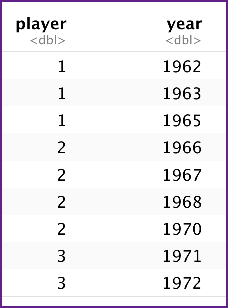
In the diagram below, data is shown for three players. The stint (number of years) shown in the year column is consecutive for only Player 3. Player 1 did not play in the season after his second year, and Player 2 skipped a season after his third year.
Input
Below is how the output looks. Player 1 skipped a year after his 1963 season, which is why in the yrDiff column there is a 2. Player 2 played continuously from his first thru third years, so a “1” is in the yrDiff column for each of those years, but did not play in 1969, thus there is a two-year gap between 1968 and 1970. Player 3 played continuously during his two years with the team.
Output

player_data %>%
  mutate(yrDiff=ifelse (is.na( year - lag(year)),1, year - lag( year )))
In this code, dplyr is used. The mutate function will create a new variable named yrdiff. To create the value for yrdiff, it seeks both the first value in year (1962) and the previous year’s value — seeking that using lag; however, as 1962 is the first data item in the column, nothing precedes it so nothing can be subtracted from 1962. Therefore, the is.na check, which asks, “Is a previous year Not Available?”, returns TRUE. When the is.na result is true, yrDiff displays 1; whereas, when it is false, which means lag(year) found a number, yrDiff displays the year – lag(year) result.
To represent the input in R, you need the code below.
Input Code
player_data <- data.frame(player = c(1,1,1,2,2,2,2,3,3), year = c(1962,1963,1965,1966,1967,1968,1970,1971,1972))
Let’s look at a real-world example. I recently investigated several baseball-related questions that shows the power of R. I obtained the data from stathead.com, formatted it in Apple Numbers, and then imported it into RStudio. The dataset contained 657 observations.
Among the results I obtained was how many games each pitcher started. This R code accomplished that:
allStarters |>
  group_by(Player) |>
  summarize(SumSt = sum(GS)) |>
  arrange(desc(SumSt))
Tom Seaver started 395 games, followed by Jerry Koosman with 346 starts and Dwight Gooden with 303. No other Mets’ pitcher had 300-plus starts.
To learn how many starts each pitcher had, I grouped each one’s data.
allStarters |>
   group_by(Player)
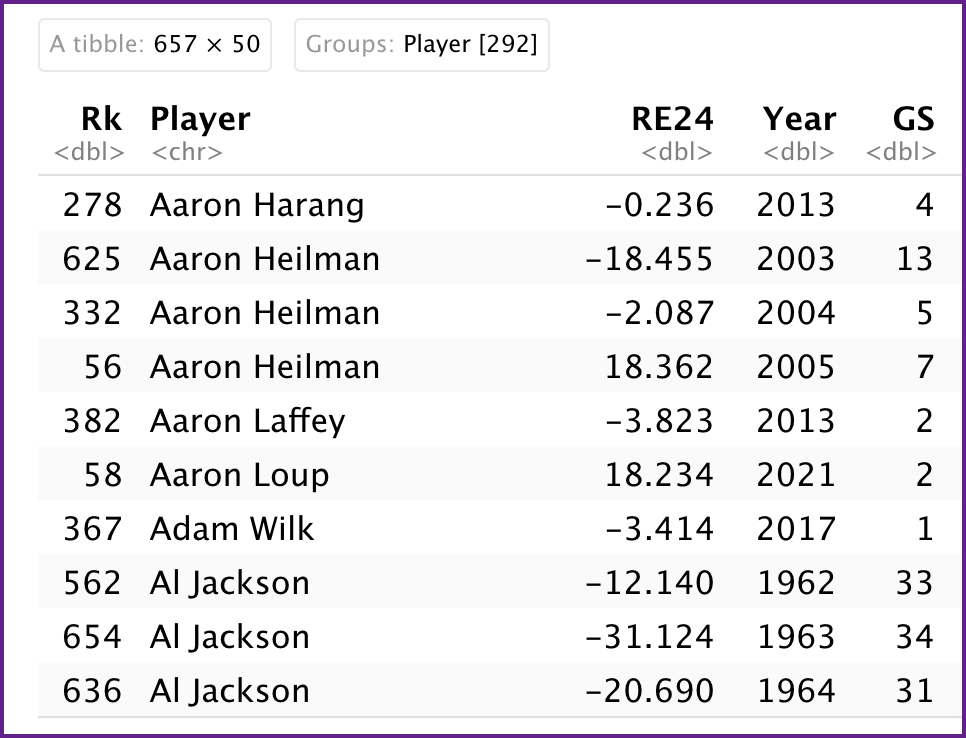
Two hundred ninety two pitchers were grouped by season with the years they started games arranged in ascending order. The diagram below contains a sample of part of one output display.
Next, I included the previously discussed mutate code to determine for each pitcher which years were consecutive.
allStarters |>
   arrange(Player, Year) |>
   group_by((Player)) |>
   mutate(yrDiff=ifelse(is.na(Year - lag(Year)),1,Year - lag(Year))) |>
   relocate(yrDiff, .after = Year)
Here is a sample of that code’s output:

In the first yrDiff column for Al Jackson, the “1” means that he started games in 1965 and that 1965 was either the first season he started for the Mets or that he also started games in 1964; whereas, the “3” in the yrDiff column for 1968 means that it had been three seasons since he last started a Mets game.
R is a great tool for those interested in doing the statistical analysis of baseball data. To use R effectively, there is a lot to learn; however, I have found the payoff to be well worth the effort expended to get it.
1 It is assumed that you have had some interaction with R or another programming language.
